Additional LP Applications

MGMT 306

Alex L. Wang

Purdue University

FloatAway Tours

Product Mix LP example

Problem Description

• Boat rental service has $420,000 for new boats
• Two different manufacturers: Sleekboat and Racer
• The new fleet must satisfy:
  • At least 50 boats total
  • Same number of boats from each manufacturer (goodwill)
  • Total seating capacity at least 200
• Formulate an LP model to maximize total expected daily profit

Boat	Manufacturer	Cost	Seats	E. Daily Profit
Speedhawk	Sleekboat	$6,000	3	$70
Silverbird	Sleekboat	$7,000	5	$80
Catman	Racer	$5,000	2	$50
Classy	Racer	$9,000	6	$110

Instructions

• As a class
  • Write an LP model for this problem
• In pairs
  • Solve the LP model in Excel
  • Output a Sensitivity Report and an Answer Report
  • Check your Excel output matches the following slides

LP Model Decision Variables and Objective

Decision variables

\[\begin{aligned} &x_1&&\text{number of Speedhawks to purchase}\\ &x_2&&\text{number of Silverbirds to purchase}\\ &x_3&&\text{number of Catmans to purchase}\\ &x_4&&\text{number of Classies to purchase} \end{aligned}\]

Objective

\[\max\; 70x_1 + 80x_2 + 50x_3 + 110x_4 \quad \text{(expected daily profit)}\]

LP Model Constraints

Constraints

\[\begin{aligned} &6000x_1 + 7000x_2 + 5000x_3 + 9000x_4 \le 420000 &&\text{(budget)}\\ &x_1 + x_2 + x_3 + x_4 \ge 50 &&\text{(at least 50 boats)}\\ &x_1 + x_2 - x_3 - x_4 = 0 &&\text{(goodwill)}\\ &3x_1 + 5x_2 + 2x_3 + 6x_4 \ge 200 &&\text{(seat capacity)}\\ &x_i \ge 0 \qquad\text{for all }i=1,2,3,4 && \text{(nonnegativity)} \end{aligned}\]

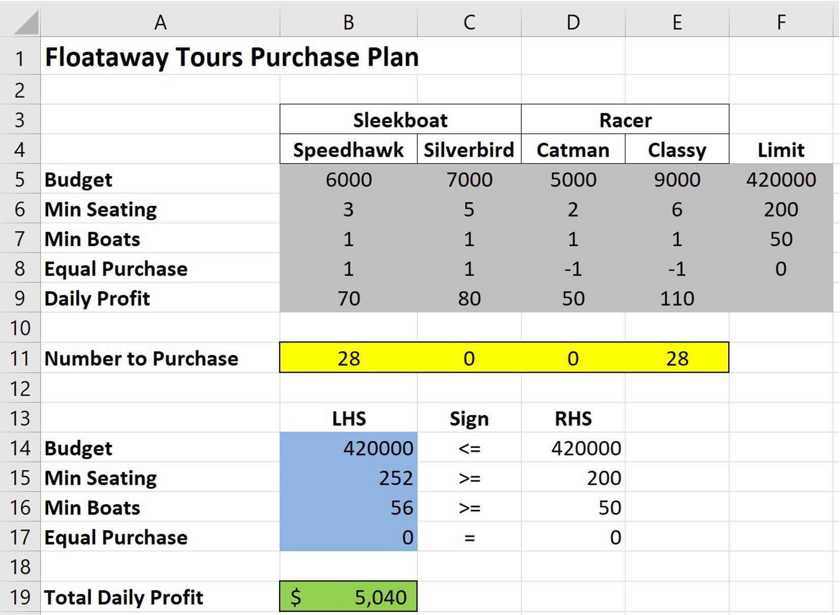
Excel Model

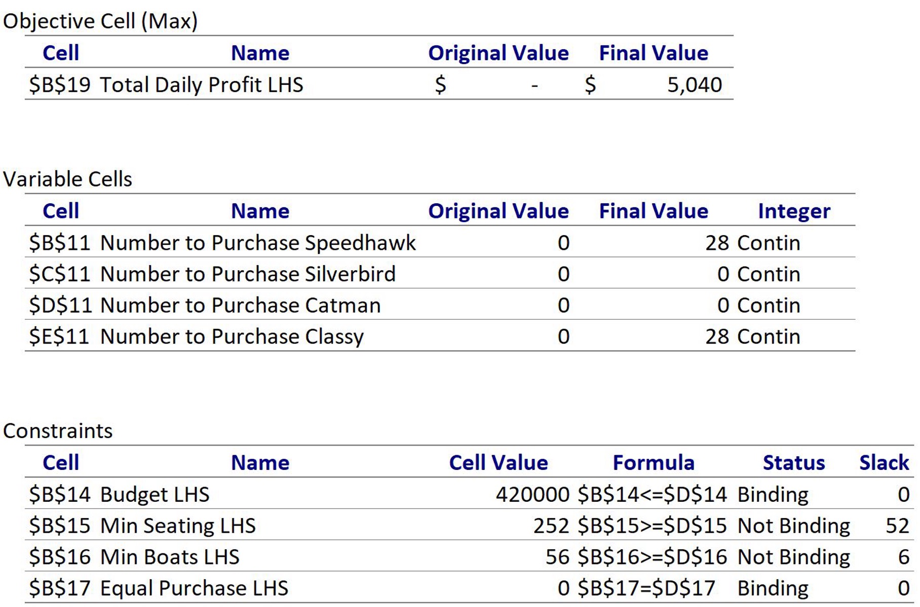
Answer Report

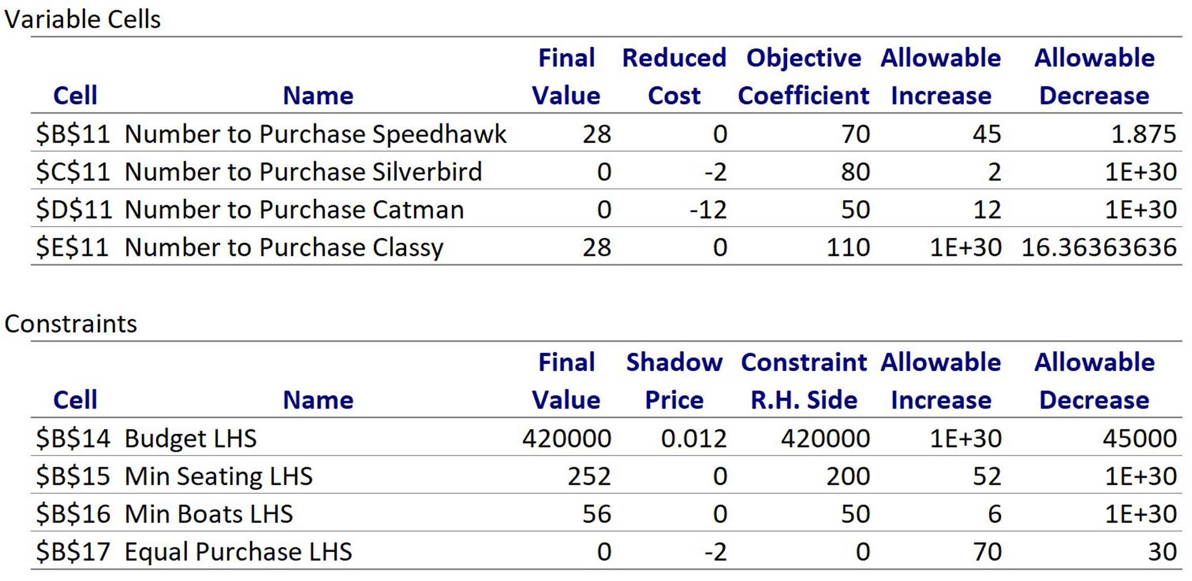
Sensitivity Report

Sensitivity Analysis Problem 1

Question. How much does the unit expected profit per Silverbird need to increase before you can justify buying Silverbirds?

Solution.

• The reduced cost of Silverbirds is -2.
• Interpretation: each Silverbird purchased would currently decrease expected daily profit by $2.
• So the expected daily profit for Silverbirds must increase by $2 to break even and justify purchasing them

Sensitivity Analysis Problem 2

Question. How much would the total expected daily profit increase if the budget is increased by \(20{,}000\)?

Solution.

• Budget RoF: \([375{,}000,\infty)\).
• New budget: \(420{,}000 + 20{,}000 = 440{,}000\) (within the RoF).
• Shadow price of budget constraint: 0.012

\[\text{change in total expected profit} = 20{,}000\times 0.012 = 240\]

CustomBikes Planning

Multi-Period Production example

Problem Description

• CustomBikes produces men’s and women’s bikes and need a production/inventory schedule for the next two months:
  • how many of each model to produce in each month, and
  • how many of each model to hold in inventory at the end of each month.

Model	Production Cost	Labor Required	Current Inventory	Demand Month 1	Demand Month 2
Men’s	$120	4	20	150	200
Women’s	$90	2	30	125	150

Problem Description Continued

• Additional details:
  • Policy: total labor hours cannot increase or decrease by more than 100 hours from month to month
  • Last month: 1,000 total labor hours
  • Inventory holding cost: 2% of production cost
  • At end of month 2, should have at least 25 units of each model in inventory

Write an LP Model to minimize total production + inventory holding cost.

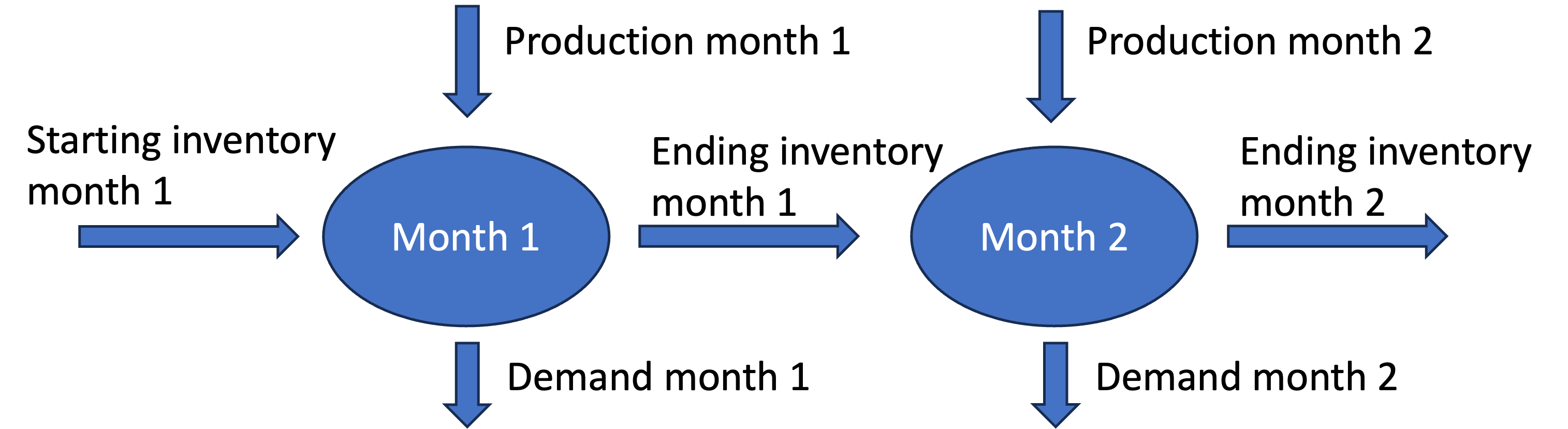
Format of multi-period production planning LPs

• This is an instance of multi-period production planning
• To set up an LP model, for each item and each time period define:
  • a production variable, and
  • an ending inventory variable.
• Write balance constraints (for each item, each time period): \[\text{Starting inv} + \text{Production} - \text{Demand} = \text{Ending inv}\]

LP Model Decision Variables and Objective

Decision variables

\[\begin{aligned} &M_i&&\text{m's bikes produced in month $i$ for } i=1,2\\ &W_i&&\text{w's bikes produced in month $i$ for } i=1,2\\ &IM_i&&\text{m's bikes in inv. at end of month $i$ for } i=1,2\\ &IW_i&&\text{w’s bikes in inv. at end of month $i$ for } i=1,2 \end{aligned}\]

Objective

\[\begin{aligned} \min\quad &120(M_1+M_2) + 90(W_1+W_2)\\ +&2.4(IM_1+IM_2) + 1.8(IW_1+IW_2) \qquad\text{(Total cost)} \end{aligned}\]

LP Model Constraints

• Total labor hours cannot increase or decrease by more than 100 hours from month to month

  \[\begin{aligned} &4M_1 + 2W_1 \le 1100\\ &4M_1 + 2W_1 \ge 900\\ &-4M_1 - 2W_1 + 4M_2 + 2W_2 \le 100\\ &-4M_1 - 2W_1 + 4M_2 + 2W_2 \ge -100 \end{aligned}\]

• At end of month 2, should have at least 25 units of each model in inventory

  \[\begin{aligned} &IM_2 \ge 25\\ &IW_2 \ge 25 \end{aligned}\]

LP Model Constraints - Men’s Bikes Balance Constraints

• Balance constraints for men’s bikes

  \[\begin{aligned} &20 + M_1 = IM_1 + 150 &&\text{(m's month 1 balance)}\\ &IM_1 + M_2 = IM_2 + 200 &&\text{(m's month 2 balance)} \end{aligned}\]

  Note Not yet in standard form

LP Model Constraints - Women’s Bikes Balance Constraints

• Balance constraints for women’s bikes

  \[\begin{aligned} &30 + W_1 = IW_1 + 125 &&\text{(w's month 1 balance)}\\ &IW_1 + W_2 = IW_2 + 150 &&\text{(w's month 2 balance)} \end{aligned}\]

  Note Not yet in standard form

Instructions

• In pairs
  • Solve the LP model in Excel
  • Output a Sensitivity Report and an Answer Report
  • Check your Excel output matches the Excel handout

Sensitivity Analysis Practice Question 1

Question. A bicycle retailer inquires about placing an order for 110 men’s bicycles in month 1 for $12,000. Should we sign a contract?

Solution

• Increasing men’s month-1 demand by 110 increases the RHS of the men’s month-1 balance constraint by 110
• This is outside RoF so shadow price formula is overly optimistic
• Since this is a minimization problem, \[\text{change in optimal cost} \geq 110\times 119.4 = 13{,}134\]
• We should not sign the contract.

Sensitivity Analysis Practice Question 2

Question. If the required inventory of women’s bicycles at the end of month 2 is 15 instead of 25, how much do we save?

Solution

• This change is within the allowable decrease for the Women’s Ending Inventory constraint.
• Cost change: \((-10)\times 91.2 = -912\).
• Total costs decrease by \(912\).

Sensitivity Analysis Practice Question 3

Question. The current inventory (end of month 0) of men’s bikes increases by 10. What is the new optimal cost and how many women’s bikes are held in inventory at the end of month 1 in the new solution?

Solution

• Increasing the current inventory of men’s bikes by 10 will decrease the right hand side of m’s month 1 balance constraint
• A decrease of 10 is within the range of feasibility, so \[\text{change in optimal cost} = (-10)\times (119.4) = -1194\]

• Since this change is within the range of feasibility, the binding constraints do not change: \(IW_1=0\)

Carter Inc. Problem

Multi-Period Production Planning example

Problem Description

From Textbook (Ch. 4, Problem 13)

• Carter Inc. is launching an energy bar in two flavors
• Demand for the next 3 months is given
• Resource requirements (peanuts, baking time) and costs are given
• Ending inventory at end of Month 3 should equal the initial inventory in Month 1

Task: formulate an LP to minimize total cost, build a spreadsheet model, and use Solver to find the optimal production and inventory schedule.

Multi-period production planning example

Demand (bars)

	Month 1	Month 2	Month 3
Peanut Power	30000	50000	40000
Peanut Crunch	80000	100000	70000

Requirements, costs, and initial inventory

	Peanuts (grams/bar)	Baking time (hours/bar)	Prod. Cost ($/bar)	Holding Cost ($/bar)	Initial Inventory (bars)
Peanut Power	60	0.01	2	0.10	10000
Peanut Crunch	40	0.015	2.5	0.15	20000

Cash Flow Planning

Problem Description

• Riverbend Capital Partners (RCP) is planning its investments for the next three years

• Currently, RCP has $2.5M available for investment

• RCP expects the following income stream from previous investments 1, 2, and 3 years from now:

  End of Year	1	2	3
  Income ($M)	$0.9	$0.75	$0.6

• There are three projects that RCP may participate in (fully or fractionally). Each project has projected cash flows for full participation.

  End of Year	0	1	2	3
  Project A Cash Flow	-3.6	-0.9	0.7	6.0
  Project B Cash Flow	-1.6	0.4	0.5	2.1
  Project C Cash Flow	-2.7	-1.5	1.1	6.7

Problem Description (continued)

• RCP can borrow money at 8% interest per year, but cannot borrow more than $2M at any point in time
• RCP can also invest surplus funds at 5% per year
• Use an LP model to maximize ending wealth at the end of three years

Variables

\[\begin{aligned} &x_A&&\text{participation in Project A}\\ &x_B&&\text{participation in Project B}\\ &x_C&&\text{participation in Project C}\\ &y_0&&\text{amount invested at end of year 0}\\ &y_1&&\text{amount invested at end of year 1}\\ &y_2&&\text{amount invested at end of year 2}\\ &z_0&&\text{amoung borrowed at end of year 0}\\ &z_1&&\text{amoung borrowed at end of year 1}\\ &z_2&&\text{amoung borrowed at end of year 2}\\ &w && \text{wealth at end of year 3} \end{aligned}\]

LP Model

• Objective: \[\max\qquad w \qquad\text{(wealth at end of year 3)}\]
• Constraints: \[\begin{aligned} &x_A \leq 1 &\text{(participation in Project A)}\\ &x_B \leq 1 &\text{(participation in Project B)}\\ &x_C \leq 1 &\text{(participation in Project C)}\\ &z_0 \leq 2 &\text{(maximum loan amount year 0)}\\ &z_1 \leq 2 &\text{(maximum loan amount year 1)}\\ &z_2 \leq 2 &\text{(maximum loan amount year 2)}\\ &\text{all variables }\geq 0 \end{aligned}\]
  • Still missing balance constraints

Cash Flow Picture

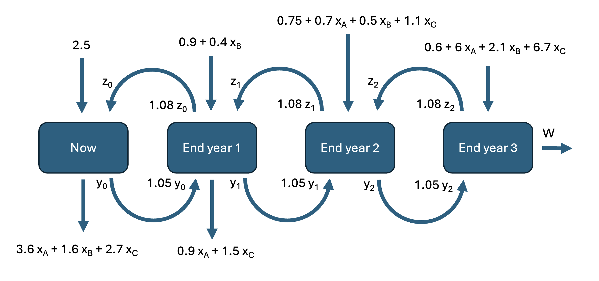
LP Model Balance Constraints

\[\begin{aligned} &2.5 + z_0 = 3.6x_A + 1.6 x_B + 2.7 x_C + y_0 &\text{(Balance 0)}\\ &0.9+0.4x_B +1.05y_0+z_1 = 0.9x_A + 1.5 x_C + y_1 + 1.08z_0&\text{(Balance 1)}\\ &0.75 + 0.7x_A + 0.5 x_B + 1.1 x_C+ 1.05 y_1 + z_2 = y_2+1.08z_1&\text{(Balance 2)}\\ &0.6 + 6 x_A + 2.1 x_B + 6.7 x_C + 1.05 y_2 = 1.08 z_2 + w &\text{(Balance 3)} \end{aligned}\]

Note: Not yet in standard form.

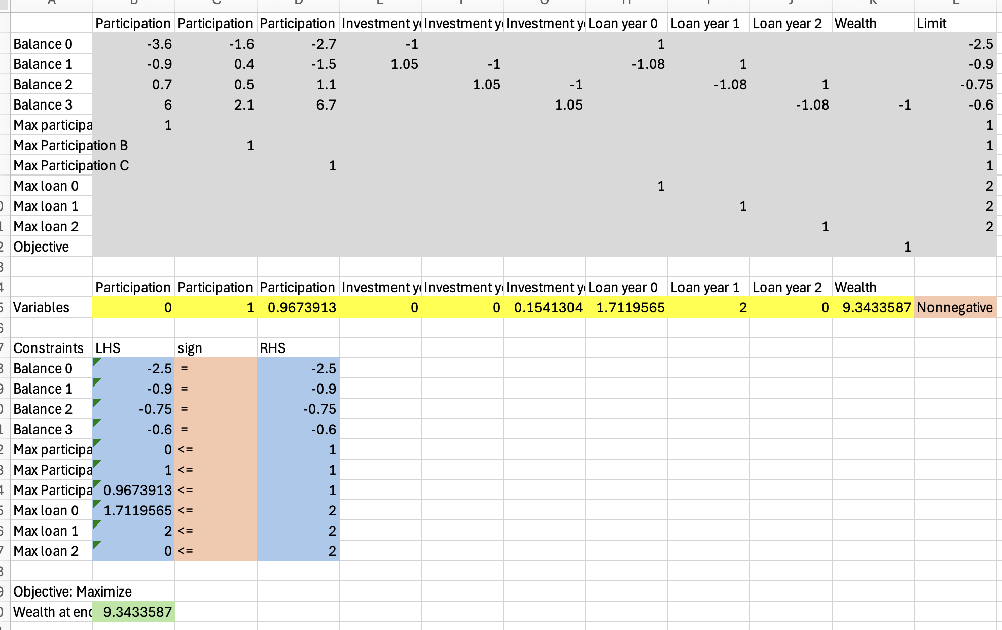
Completed Excel Spreadsheet