Two Stage Decision Analysis with LPs
MGMT 306
Purdue University
Dorothy’s farm with known yields
Problem Description
- Dorothy grows corn and sugar beets on her 320 acre farm
- Dorothy needs 240T of corn for cattle feed
- Leftover corn can be sold at $150/T
- Instead of growing the corn herself, she can buy corn for $210/T
- Beets sell for $36/T up to 5500T
- Planting costs are $230/acre and $260/acre for corn, beets respectively
- For now, assume that each acre of corn yields 3T of corn and each acre of beets yields 20T of beets
- How much of each crop should Dorothy plant / sell / buy to maximize profit?
LP Formulation
Variables \[ \begin{aligned} &p_C, p_B &&\text{acres of corn and beets to plant}\\ &s_C, s_B &&\text{tonnes of corn and beets to sell}\\ &b_C &&\text{tonnes of corn to buy} \end{aligned} \]
Objective \[ \max \quad 150s_C + 36 s_B -230 p_C - 260 p_B -210 b_C \qquad\text{(net profit)} \]
LP Formulation continued
Constraints \[ \begin{aligned} &p_C+ p_B\leq 320 &&\text{(land)}\\ &-3p_C+s_C-b_C\leq -240 &&\text{(corn yield)}\\ &-20p_B + s_B\leq 0 &&\text{(beet yield)}\\ & s_B\leq 5500 && \text{(beet sales)}\\ & \text{all variables} \geq 0 \end{aligned} \]
Explanation: The corn yield constraints says that we need to plant and buy enough corn to cover the amount we plan to sell plus the 240 required for cattle feed: \(240 + s_C \leq 3 p_C + b_C\)
The beet yield constraint is similar
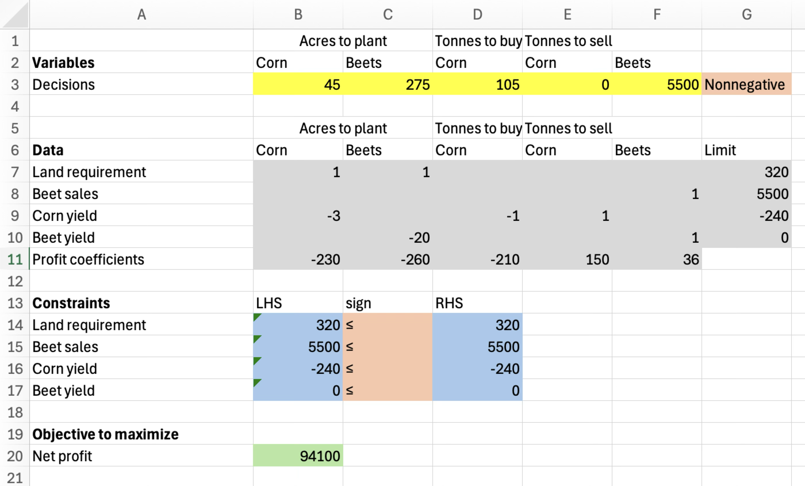
Excel model
Dorothy’s farm with uncertain yields
Problem Description
- Yield actually varies from year to year due to weather conditions
- There are three scenarios
| Scenario | Corn yield (T/acre) | Beet yield (T/acre) | Probability |
|---|---|---|---|
| 1. Good weather | 3.6 | 24 | 1/3 |
| 2. Normal weather | 3 | 20 | 1/3 |
| 3. Bad weather | 2.4 | 16 | 1/3 |
Sequence of decisions
- Decision making timeline:
- Stage 1: Dorothy plants crops (makes choices for \(p_C\), \(p_B\))
- Yield is realized (one of the three scenarios is revealed)
- Stage 2: After observing the yield, Dorothy buys deficient corn / sells surplus corn
- What should Dorothy do to maximize expected profit?
LP Model Variables
- Previously, we had five variables: \(p_C\), \(p_B\), \(s_C\), \(s_B\), \(b_C\)
- We will keep the stage 1 variables: \(p_C\), \(p_B\)
- We will replace the stage 2 variables with one copy of the stage 2 variables for each possible scenario: \[\begin{aligned} &s_{C,i}, s_{B,i}&&\text{for $i=1,2,3$}&& \text{t. of corn, beets to sell in scenario $i$}\\ &b_{C,i}&&\text{for $i=1,2,3$}&& \text{t. of corn, beets to buy in scenario $i$} \end{aligned}\] This represents how Dorothy plans to react in stage 2 to the possible weather and yield scenarios. For example, \(s_{C,1}\) is the tonnes of corn Dorothy plans to sell if there is good weather
LP Model Objective
Expected net profit: \[\begin{aligned} \max \quad& (1/3)\times\left(150 s_{C,1} + 36 s_{B,1} - 230 p_C - 260 p_B - 210 b_{C,1}\right)\\ +&(1/3)\times\left(150 s_{C,2} + 36 s_{B,2} - 230 p_C - 260 p_B - 210 b_{C,2}\right)\\ +&(1/3)\times\left(150 s_{C,3} + 36 s_{B,3} - 230 p_C - 260 p_B - 210 b_{C,3}\right) \end{aligned}\]
This is the average of the net profits in each scenario
LP Model Constraints
- Land requirement \[ p_C + p_B \leq 320\]
- Beet sales limit \[ s_{B,i} \leq 5500\quad\text{for all }i=1,2,3\]
- Nonnegativity on all varialbes
LP Model Constraints (continued)
Corn yield: \[\begin{aligned} &-3.6 p_C - b_{C,1} + s_{C,1} \leq - 240&&\text{(corn yield-1)}\\ &-3 p_C - b_{C,2} + s_{C,2} \leq - 240&&\text{(corn yield-2)}\\ &-2.4 p_C - b_{C,3} + s_{C,3} \leq - 240&&\text{(corn yield-3)} \end{aligned}\]
Beet yield: \[\begin{aligned} &-24 p_B +s_{B,1} \leq 0&&\text{(beet yield-1)}\\ &-20 p_B +s_{B,2} \leq 0&&\text{(beet yield-2)}\\ &-16 p_B + s_{B,3} \leq 0&&\text{(beet yield-3)} \end{aligned}\]
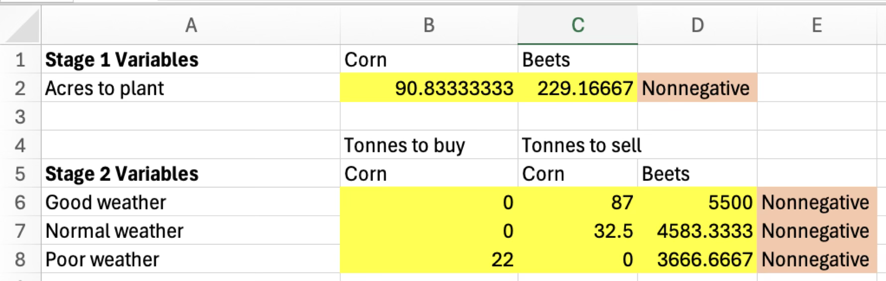
Excel model
- Split variables into stage 1 and stage 2
- Repeat stage 2 variables for each scenario
- Repeat constraint and objective calculations once for each scenario (with updated yield parameters)
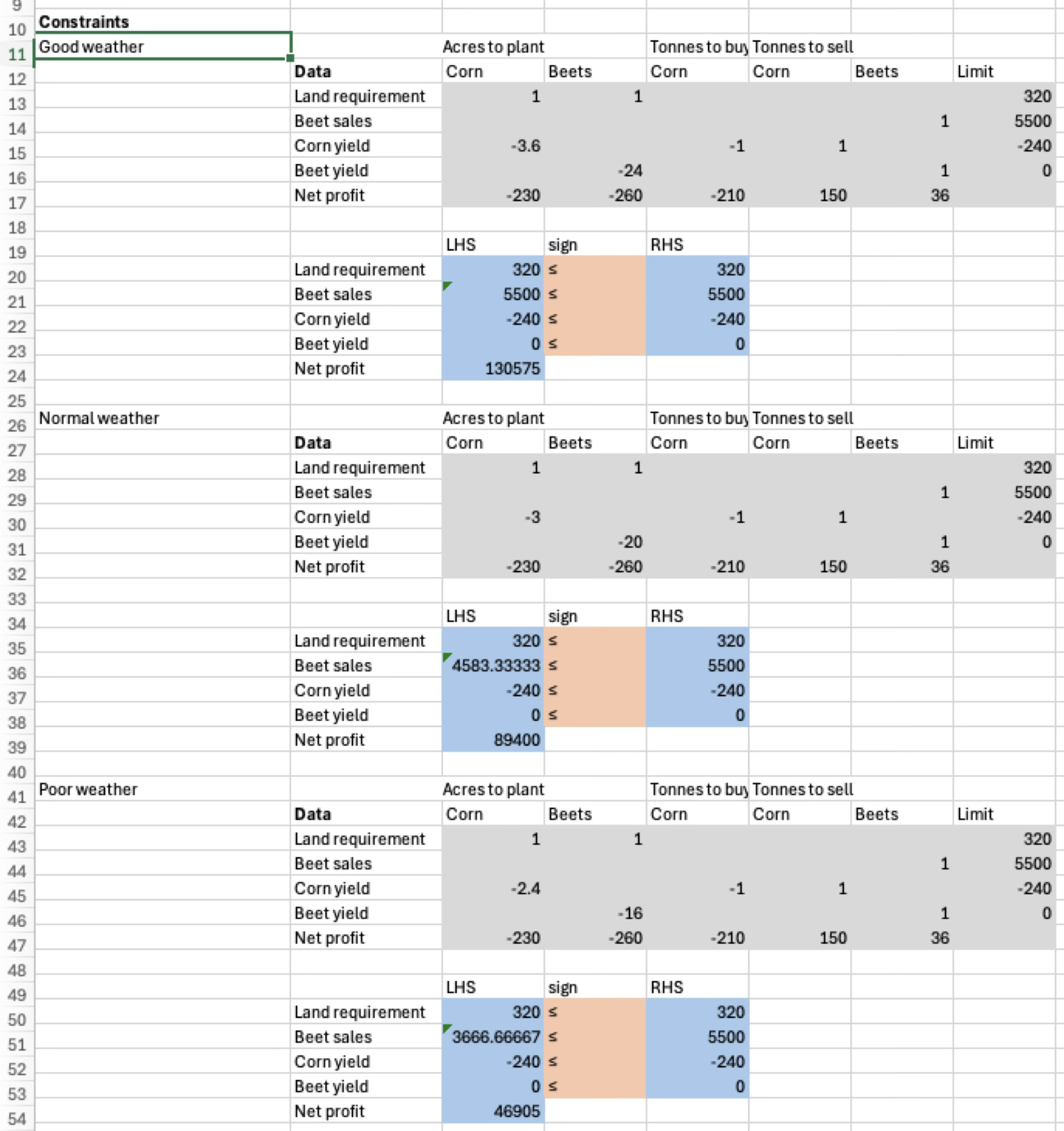
Excel model (continued)
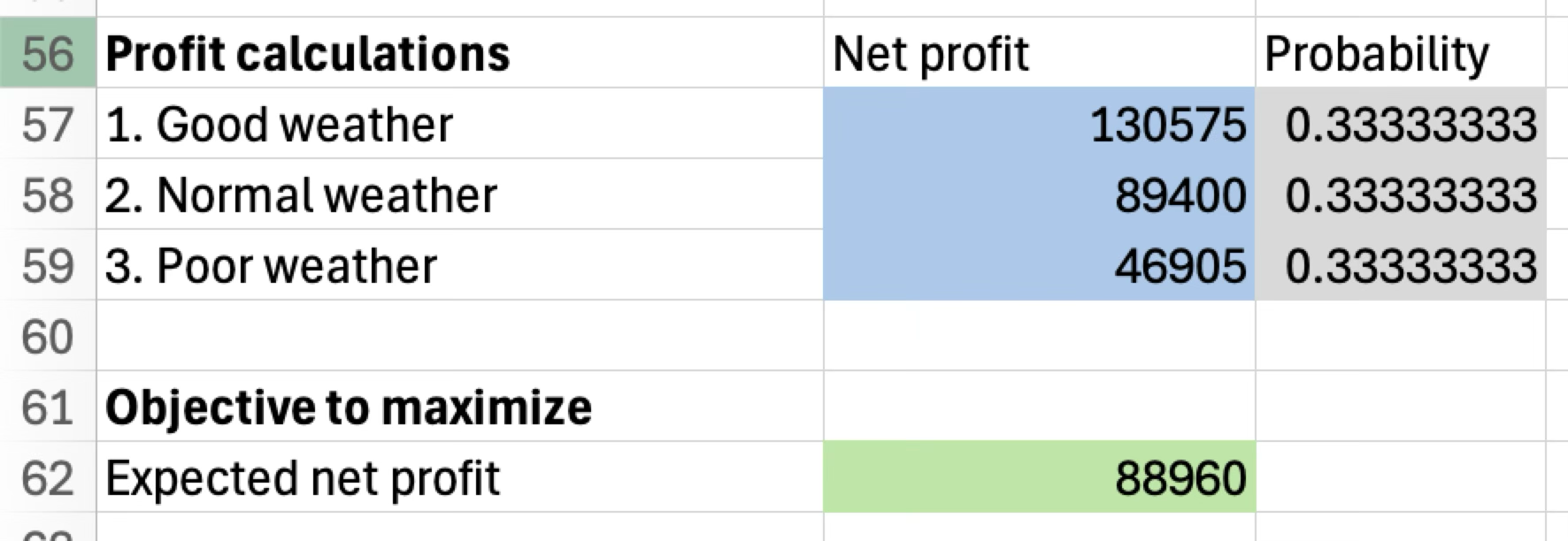
- Set objective to the average of the three profit values
- The Expected Value (EV) is $88,960
Expected Value of Perfect Information (EVPI)
- Recall that EVPI is the difference between Expected Value with Perfect Information (EVwPI) and the expected value (EV)
- We can use the same spreadsheet with different probabilities to compute the EVwPI
- Scenario 1: $130,575
- Scenario 2: $94,100
- Scenario 3: $50,720
- The EVwPI is \(\text{EVwPI} = \frac{1}{3}\cdot 130575 + \frac{1}{3} \cdot 94100 + \frac{1}{3}50720 =91789.33\)
- The EVPI is \(\text{EVPI} = \text{EVwPI} - \text{EV} = 2829.33\)
Practice Problems
Lakeshore Outdoor Gear
- Lakeshore Outdoor Gear, an outdoor equipment retailer, must decide how many camping tents to stock before the summer season starts
- The demand for tents is uncertain, but the marketing department reports three demand scenarios
- If the demand exceeds the initial inventory, Lakeshore Outdoor Gear may fulfill additional orders by purchasing emergency inventory at a “last-minute” stocking cost
- If the demand is lower than their initial inventory, then at the end of the season, Lakeshore Outdoor Gear will put the remaining inventory on sale.
- All relevant data is shown on the next page
Lakeshore Outdoor Gear (Continued)
| Scenario | In-season demand | Sale demand |
|---|---|---|
| Scenario 1 | 200 | 40 |
| Scenario 2 | 150 | 40 |
| Scenario 3 | 100 | 40 |
| Timing | Cost |
|---|---|
| Initial stocking cost | $50/tent |
| Last-minute stocking cost | $75/tent |
| Timing | Revenue |
|---|---|
| In-season (Normal) price | $80/tent |
| End-of-season (Sale) price | $40/tent |
Lakeshore Outdoor Gears Instructions
- Write an LP model to maximize profit assuming Scenario 1
- Implement the LP model from Part a. in the same Excel sheet and use it to compute the PWPI
- Duplicate the previous sheet. Modify it assuming Scenario 2
- Duplicate the previous sheet. Modify it assuming Scenario 3
- In a new sheet, write a two-stage LP model to maximize expected profit
- Implement the LP model from part e. in the same Excel sheet and use it to compute the EV
- Compute the EVWPI and EVPI
Whisked Away Bakery
- Whisked Away Bakery is an order-only bakery selling chocolate cakes
- Avery, the manager of Whisked Away Bakery, plans each day’s operations three days out
- Today (a Monday), Avery must:
- Order fresh butter and eggs from their supplier at a cost of $3.50/lb butter and $0.15/egg
- Schedule Thursday’s hours for the bakers at a rate of $15/hour up to a maximum of 12 hours
- Each cake requires 1/3 hours of labor, 1/4 lb of butter, and 4 eggs
- The remaining shelf-stable ingredients cost $4.15 per cake
- Each cake sells for $25.00
Whisked Away Bakery (continued)
- Avery believes there are two possible scenarios for the number of orders they will receive
| Scenario | Number of orders | Probability |
|---|---|---|
| 1. High demand | 50 | 50% |
| 2. Low demand | 30 | 50% |
- After the order form closes on Wednesday night, Avery may then
- Purchase additional butter and eggs at the retail price: $6.00/lb butter and $0.30/egg
- Schedule last-minute staff at a rate of $20/hour
- Whisked Away Bakery must fulfill all orders they receive
- How can Avery maximize the expected profit?
Whisked Away Bakery Instructions
- Write an LP model to maximize profit assuming Scenario 1
- Implement the LP model from Part a. in the same Excel sheet and use it to compute the PWPI
- Duplicate the previous sheet. Modify it assuming Scenario 2
- In a new sheet, write a two-stage LP model to maximize expected profit
- Implement the LP model from part d. in the same Excel sheet and use it to compute the EV
- Compute the EVWPI and EVPI